Desorption

In my work, I have studied desorption using two different methods: bond-boost method and temperature acceleration method. The bond-boost method is described in detail in its own section in this website. Below, I describe the temperature acceleration method with a simple example, that implicitly uses umbrella sampling of the data.

Temperature Acceleration

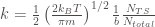
Desorption at low temperature is a rare event that cannot be sampled sufficiently by regular MD (over computationally tractable time period). Therefore, one way of simulating desorption is by employing accelerated MD via the temperature acceleration method. This method is based on sampling high-energy configurations using umbrella sampling. However, instead of applying a bias potential to perform high-energy sampling, the simulation is conducted at a high temperature where desorption occurs rapidly enough to allow sufficient sampling over a tractable computation period. Using the data sampled, the rate constant is calculated using the equation derived in this page:

$k_{fwd} = \frac{1}{2} \left( \frac{2 k_B T}{\pi m} \right)^{1/2} \frac{\int\delta(\mathbf{R-R^*}) \exp(-U(\mathbf{R})/k_B T) d\mathbf{R}}{\int \exp(-U(\mathbf{R})/k_B T) d\mathbf{R}}\label{eq:k_fwd}$

where the integral at the numerator represents the canonical average at the infinitesimally thin transition state (TS) identified by $\mathbf{R}{^*}$ , the integral at the denominator represents the canonical average over all space, U( $\mathbf{R}$ ) represents the adsorbate-substrate potential and m represents the mass of adsorbate. Assigning a finite width $\textsl{b}$ to the TS, the above equation simplifies to

$k = \frac{1}{2} \left( \frac{2 k_B T}{\pi m} \right)^{1/2} \frac{1}{b} \frac{N_{TS}}{N_{total}}$

where $N_{TS}$ is the number of iterations spent in TS and $N_{total}$ is the total number of iterations.

The rate constant calculated from the above setup will provide the rate constant at the high temperature employed. In order to obtain the rate constant at the original temperature, we use a weighting function $W(\mathbf{r})$ implemented in the transition-state theory equation:

$k = \frac{1}{2b} \left( \frac{2 k_B T}{\pi m} \right)^{1/2} \frac{\int\delta(\mathbf{R-R^*}) W(\mathbf{R}) \exp(-U(\mathbf{R})/k_B T) d\mathbf{R} / W(\mathbf{R})}{\int W(\mathbf{R}) \exp(-U(\mathbf{R})/k_B T) d\mathbf{R} / W(\mathbf{R})}$

The form of $W(\mathbf{R})$ can be chosen as required to facilitate the evaluation of the above equation. Choosing $W = \exp \left( \frac{U(\mathbf{R}) - U^*(\mathbf{R})}{k_B T} \right)$ , where $U^*(\mathbf{R})$ is the modified potential energy surface traversed by molecules at the increased temperature, we get:

$k = \frac{1}{2} \sqrt{\frac{2 k_B T}{\pi m}} \frac{1}{b} \frac{<\delta(\mathbf{R-R^*})/W>_{U*}}{<1/W>_{U^*}}$

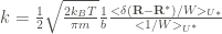
The subscript $U^*$ indicates that the energy of the system was sampled from the modified potential surface created at the higher temperature.

Let us suppose that the $s$ is scaling factor that represents the increase in temperature, i.e. $s = T^*/T$ where $T$ is the original temperature and $T^*$ is the higher temperature. Accordingly, potential energy surface is modified to become $U^* = U/s$ . Then, the weighting function becomes:

$W = \exp \left[ -\frac{s-1}{s} \frac{U(\mathbf{R})}{k_B T} \right]$

In practice, the value of $s$ is chosen in the range $\approx$ 2 to prevent excessive biasing (see theory section).

Example: 1D Desorption

Simulation

[Click here for code]

A 1D Morse potential $V_{1D}$ is constructed: $V_{1D}(x) = D_e \left[(1-e^{-\alpha(x-x_{0})})^2-1 \right]$

where $D_e = 0.0109 \ eV$ , $\alpha = 2.4 \ \AA^{-1}$ and $x_0 = 1.5 \ \AA$ .

The minimum of this potential at $x = 1.5 \ \AA$ represents the surface, and a transition region is implemented at $x = 4.5 \ \AA$ of width $b = 0.1 \ \AA$ . A reflecting wall is located immediately beyond the transition region. A single point particle of mass $m = 4.146 \times 10^{-3} \ eV ps^2 / \AA^2$ is introduced into this 1D system. The particle is thermostated using an Andersen thermostat of velocity generation frequency $nu=0.01$ . It is active only in the region $x < 1.6 \ \AA$ to model thermostating near the surface. The trajectory of the particle is calculated using a Verlet algorithm. Using a timestep of 1 fs, desorption of the particle is simulated at 25 K using the temperature acceleration methods, with a temperature scaling of $s = 2.0$ , over $5 \times 10^6$ iterations.

The rate constant is calculated at 25 K using the equation described in the above section.

Theoretical Calculation

[Click here for code]

In addition, the occupation probability distribution $P(x)$ of this potential is caclculated from the simulation data. In the original system, $P(x+\Delta x)$ is simply the ratio of number of iterations spent in interval $x+\Delta x$ , $N(x+\Delta x)$ , to the total number of iterations, $N_{total}$ , i.e.

$P(x+\Delta x) = \frac{N(x+\Delta x)}{N_{total}}$

The occupation probabilities of every $0.1 \AA$ interval, i.e. $P(x+0.1 \AA)$ , are calculated for both bond-boost and temperature acceleration methods, where the weighting factors are incorporated using:

$P_{TempAcc}(x+\Delta x) = \frac{ \sum \limits_{i=1}^{N(x+\Delta x)} \exp{\left[-\frac{s-1}{s} \frac{V_{1D}(x_i)}{k_B T} \right]}}{\sum \limits_{i=1}^{N_{total}} \exp{\left[-\frac{s-1}{s} \frac{V_{1D}(x_i)}{k_B T} \right]}}$

for temperature acceleration, where $x_i$ represents the position of the particle at the $i$ th iteration.

In addition, the theoretical rate constant $k_{theory}$ and occupation probability distribution $P_{theory}(x)$ are numerically calculated from the potential profile:

$P_{theory}(x+0.1 \AA) = \frac{\int_x^{x+0.1 \AA}\exp{\left(-V_{1D}(x)/k_B T\right)}dx}{\int_0^{x = 4.6 \AA}\exp{\left(-V_{1D}(x)/k_B T\right)}dx}$

$k_{theory} = \frac{1}{2} \sqrt{\frac{2 k_B T}{\pi m}} \frac{1}{b} \frac{\int_{4.5 \ \AA}^{4.6 \ \AA}\exp{\left(-V_{1D}(x)/k_B T\right)}dx}{\int_0^{4.6 \AA}\exp{\left(-V_{1D}(x)/k_B T\right)}dx}$

P(x).png — The probability distributions for the 1D Morse potential obtained theoretically (blue) and by temperature-acceleration (green). The three plots are seen to overlap over the entire range, indicating reasonable match with each other.

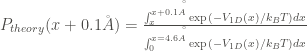
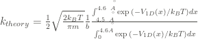
The comparison of $P_{theory}(x)$ with $P(x)$ obtained from the two simulations are shown in the above figure. It is observed that the $P(x)$ compares very well with $P_{theory}(x)$ , as do the simulated rate constants with $k_{theory}$ ( $k_{TempAcc} = (4.47 \pm 0.17) \times 10^{-3} \ ps^{-1}$ , $k_{theory} = 4.70 \times 10^{-3} \ ps^{-1}$ ) .

Note: however, it must be pointed out that the temperature acceleration method in studying desorption is inherently flawed since the rate constant is entropy dependent, and hence temperature dependent. Therefore, by employing a large temperature, the system properties are modified and the rate constant calculated even after accounting for the bias temperature do not reflect the original rate constant. This error becomes more prominent when desorption in a system with larger degrees of freedom is studied, where entropy change from adsorption to desorption is greater, e.g. desorption of benzene (see chapter from my dissertation, pg. 31). A better method that circumvents this problem is the bond-boost method.

Temperature Acceleration

Example: 1D Desorption

Simulation

Theoretical Calculation

Share this: